Advanced Signal Decompositions Need the Right Test
SWT, synchrosqueezing, EMD, VMD, and EWT encode different assumptions. Four synthetic diagnostics show what each method earns, where a direct baseline still wins, and why one leaderboard cannot answer every regime question.
By MorphIQ Labs · Quant research
SWT, synchrosqueezing, EMD, VMD, and EWT are often placed in the same comparison table because they all decompose a signal. That makes them look like interchangeable candidates for one job. They are not.
SWT removes decimation to make a wavelet representation insensitive to sample alignment. Synchrosqueezing sharpens a redundant time-frequency map under an AM-FM component model. EMD and its ensemble variants infer oscillatory modes from extrema. VMD asks for a mode count and solves a global variational problem. EWT builds a filter bank from boundaries detected in the observed spectrum.
Asking which one "wins" before stating the signal structure and the failure being measured is a category error. This note uses four generated-signal diagnostics instead. Each has known ground truth, a fixed score, repeated random trials where appropriate, and a direct baseline.
These are transform diagnostics, not a market backtest. They use no market data, trading labels, production thresholds, or private transform rankings.
Four questions, not one leaderboard
| Diagnostic | Known structure | Methods | Primary question |
|---|---|---|---|
| Shift invariance | One signal circularly shifted by 1 through 32 samples | Decimated DWT, SWT | Does sample alignment change the scale-energy feature? |
| Time-frequency concentration | Two noisy components with known instantaneous frequencies | CWT, SSWT | How tightly does energy remain around the true ridges? |
| Noise-assisted mode separation | Two noisy modes, one intermittent | EMD, EEMD, CEEMDAN | Can distinct recovered modes preserve the known components? |
| Filter-bank contract | Three noisy stationary tones | Periodogram, VMD, EWT | What happens when mode count or boundary detection is under-, correctly, or over-specified? |

SWT and SSWT are different methods
The names are close enough to cause persistent confusion.
SWT is the stationary wavelet transform. It removes the downsampling step from the discrete wavelet transform, leaving a redundant coefficient sequence at every level. For an orthogonal wavelet with normalized coefficients, its energy can be partitioned across scales while remaining invariant to circular translation.
SSWT is the synchrosqueezed wavelet transform. It begins with a continuous wavelet transform and reassigns coefficient energy toward estimated instantaneous frequencies. Its purpose is sharper localization of sufficiently separated oscillatory components, not shift invariance of a discrete scale decomposition.
They deserve separate tests.
Test 1: what SWT buys
The first diagnostic constructs a 512-sample signal from two localized wave packets and a step. A four-level Daubechies-4 decomposition is calculated for the original signal and for 32 circular translations. The feature is the normalized energy at each detail level plus the final approximation level.
For translation , feature drift is
| Method | Mean drift | Maximum drift |
|---|---|---|
| Decimated DWT | 0.00893 [0.00742, 0.01043] | 0.01490 |
| SWT |
The SWT differences are floating-point residue. Its scale-energy feature is unchanged by the tested translations. The decimated DWT feature is not.
This is not evidence that SWT is a better transform for every task. Redundancy costs memory and computation, and boundary treatment still matters for a non-circular record. It establishes the narrower claim: if a sliding feature must not depend on even-versus-odd sample alignment, decimation introduces a failure mode that SWT removes. The same motivation underlies the use of MODWT for time-aligned scale features; PyWavelets documents SWT as closely related to MODWT when normalized.
Test 2: when synchrosqueezing earns its complexity
The second generator produces two amplitude- and frequency-modulated components. One rises from roughly 0.035 to 0.115 cycles per sample while the other moves from roughly 0.260 toward 0.195. Gaussian noise is added, and the experiment is repeated for 20 independently seeded signals.
CWT and SSWT use the same generalized Morse wavelet, the same 24 voices per octave, and the same reflected boundary treatment. Scoring excludes 72 samples at either edge. Two measurements are reported:
- Ridge energy share: energy within 0.01 cycles per sample of either true instantaneous frequency.
- Effective occupied bins: the exponential of spectral entropy,
| Method | Energy near true ridges | Effective occupied bins |
|---|---|---|
| CWT | 56.91% [56.38, 57.42] | 33.50 [33.19, 33.82] |
| SSWT | 93.90% [93.48, 94.29] | 3.88 [3.79, 3.96] |
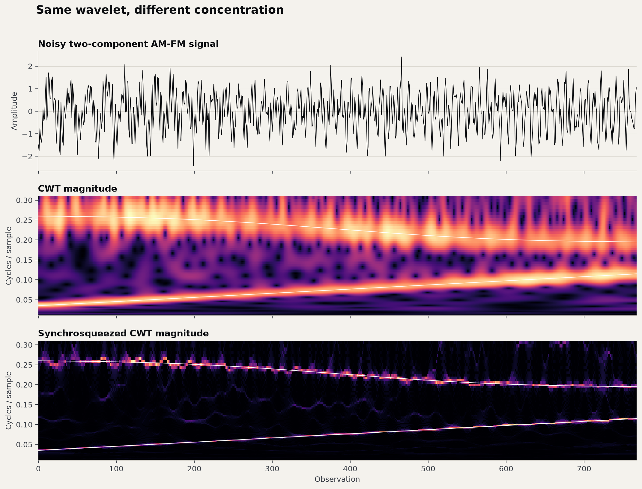
This is the kind of signal for which synchrosqueezing was built, so it should win this test. The result would be suspicious if it did not.
It does not follow that SSWT is automatically the best representation for an abrupt variance change, a jump process, or a state defined directly by lagged dependence. Synchrosqueezing assumes meaningful AM-FM components and sufficient separation. The diagnostic confirms that the implementation expresses that assumption when the generator satisfies it.
Test 3: EMD, EEMD, and CEEMDAN under mode mixing
Plain EMD constructs intrinsic mode functions by iteratively removing local envelope means. Its adaptivity is useful, but intermittency and noise can mix physical components across modes. EEMD attacks that problem by decomposing noise-perturbed copies and averaging corresponding modes. CEEMDAN uses stage-wise adaptive noise to improve completeness and reconstruction behavior.
The test signal contains a persistent low-frequency mode and an intermittent high-frequency mode under additive noise. Twenty independently seeded signals are decomposed. EEMD and CEEMDAN each use 20-member ensembles with fixed noise seeds.
Recovered modes are matched one-to-one with the two known components using a minimum-cost assignment. The score is mean squared correlation across the assigned pairs. Requiring distinct modes prevents both targets from taking credit for the same IMF.
| Method | Distinct-mode assigned |
|---|---|
| EMD | 0.603 [0.575, 0.627] |
| EEMD | 0.728 [0.720, 0.737] |
| CEEMDAN | 0.664 [0.648, 0.679] |
EEMD produces the cleanest isolation under this generator and these ensemble settings. CEEMDAN improves on plain EMD but does not lead this scorecard. That is not a contradiction: CEEMDAN's design also addresses decomposition completeness and reconstruction, while this diagnostic scores component isolation only.
The useful conclusion is not "EEMD beats CEEMDAN." It is that the benefit claimed for noise-assisted decomposition can be measured against known modes, and that a more elaborate variant does not inherit first place on every objective. Ensemble size, injected-noise scale, stopping criteria, end effects, runtime, and deterministic seeding remain part of the method contract.
Test 4: adaptive methods still need a contract
The final generator is intentionally simpler: three well-separated stationary sinusoids under noise. Frequencies and amplitudes are jittered across 24 trials. A recovered mode counts as a hit when its dominant frequency is within 0.012 cycles per sample of a known component.
Two scores are needed:
- Known-frequency recall: how many of the three true frequencies were recovered?
- Returned-mode precision: how many returned modes correspond to one of those frequencies?
| Method | Recall | Mode precision | Extra modes |
|---|---|---|---|
| Periodogram, top 3 peaks | 100.0% | 100.0% | 0.0 |
| VMD, | 66.7% | 100.0% | 0.0 |
| VMD, | 100.0% | 100.0% | 0.0 |
| VMD, | 100.0% | 75.0% | 1.0 |
| VMD, | 100.0% | 60.0% | 2.0 |
| EWT, local-max boundaries with | 59.7% [52.8, 66.7] | 59.7% [52.8, 66.7] | 0.0 |
| EWT, automatic scale-space boundaries | 100.0% | 18.8% [17.9, 19.8] | 13.21 [12.46, 13.96] |
The direct periodogram baseline solves the stationary-frequency question without a decomposition. VMD also solves it when given the correct mode count. is precise but incomplete; and retain every true component by splitting the representation into additional modes.
The two EWT boundary rules fail differently. Constraining the local-max filter bank to three bands misses known tones in some noisy trials. The default Otsu scale-space detector finds all three, but does so while returning roughly 16 modes on average. A recall-only table would have called that perfect.
This does not establish a general defect in EWT. It establishes that boundary detection, regularization, and the expected number of supports are part of the claim. "Adaptive" does not mean configuration-free, and returning more modes makes recovery easier unless precision is scored beside recall.
What belongs in a causal regime study
These diagnostics operate on complete synthetic records. EMD, VMD, EWT, CWT, and SSWT as used here can all incorporate samples to the right of an interior point. The figures therefore test representation quality, not live detection latency.
A runtime-facing regime experiment needs another layer:
- Trailing evaluation. Recompute the feature from data available at time and score only the endpoint output.
- Boundary policy. State padding, extension, warm-up, and coefficients excluded from scoring.
- Stable labels. Distinguish recognizing a state from predicting a transition.
- Switch accounting. Keep false switches and missed transitions beside conditional detection delay.
- Held-out paths or walk-forward data. Choose mode counts, boundaries, thresholds, and smoothing away from the final evaluation set.
- Compute accounting. Compare quality at the latency and throughput budget the runtime actually has.
That is the bridge from a transform that behaves correctly on canonical input to a detector that can make a defensible market claim. The companion note, How to Evaluate a Market Regime Detector Without Fooling Yourself, develops that causal scorecard on equal-variance AR(1) paths.
Why MEMD is not in this benchmark
MEMD is not represented by running EMD independently on multiple channels. Its purpose is joint mode alignment across projections of a multichannel signal. A defensible public test needs known shared modes, channel-specific modes, controlled phase offsets, channel-dependent noise, and an alignment score across channels.
That is a separate experiment. Omitting it is more accurate than using a univariate surrogate and calling the result multivariate evidence.
What this establishes
This benchmark supports four bounded claims:
- normalized SWT scale energy is translation invariant in the tested setup;
- SSWT concentrates separated AM-FM components more tightly than its source CWT under the stated score;
- noise-assisted EMD variants can improve component isolation, but their order depends on the objective and configuration;
- VMD mode count and EWT boundary selection must be scored for both recovery and over-decomposition.
It does not establish that any method predicts returns, identifies a market regime, produces an ML feature with out-of-sample value, or should be a production default.
Reproduction
The generated-signal definitions, fixed seeds, transform configurations, metrics, and plotting code are available in the benchmark script. Dependencies are pinned in requirements.txt. Unrounded aggregate results are available as CSV and JSON.
python3.12 -m venv .venv
.venv/bin/pip install -r requirements.txt
.venv/bin/python benchmark.py
The public benchmark deliberately uses widely available Python implementations
so readers can reproduce it without access to MorphIQ Labs software: PyWavelets
for DWT/SWT, ssqueezepy for CWT/SSWT, EMD-signal for the EMD family,
sktime's maintained VMD implementation, and the official pyewt package for
EWT.
MorphIQ Labs' proprietary research and runtime engineering use FerroWave, our Rust implementation of these transform families, including MODWT/SWT, CWT/SSWT, EMD/EEMD/CEEMDAN/MEMD, VMD, and EWT. FerroWave adds reference-oracle and property validation, deterministic or explicitly seeded execution, formal proofs for specifiable invariants, streaming and incremental interfaces, and benchmarked SIMD-enabled kernels. The results reported here test method-level behavior through the public Python implementations; they are not a performance comparison against FerroWave.
References
- PyWavelets, Stationary Wavelet Transform documentation.
- Ingrid Daubechies, Jianfeng Lu, and Hau-Tieng Wu, "Synchrosqueezed Wavelet Transforms: An Empirical Mode Decomposition-Like Tool", Applied and Computational Harmonic Analysis 30(2), 2011.
- Norden E. Huang et al., "The Empirical Mode Decomposition and the Hilbert Spectrum for Nonlinear and Non-Stationary Time Series Analysis", Proceedings of the Royal Society A 454, 1998.
- Zhaohua Wu and Norden E. Huang, "Ensemble Empirical Mode Decomposition: A Noise-Assisted Data Analysis Method", Advances in Adaptive Data Analysis 1(1), 2009.
- Maria E. Torres et al., "A Complete Ensemble Empirical Mode Decomposition with Adaptive Noise", ICASSP, 2011.
- Konstantin Dragomiretskiy and Dominique Zosso, "Variational Mode Decomposition", IEEE Transactions on Signal Processing 62(3), 2014.
- Jerome Gilles, "Empirical Wavelet Transform", IEEE Transactions on Signal Processing 61(16), 2013.
- Public implementations:
ssqueezepy,PyEMD,sktimeVMD, andpyewt.
More from Quant Research
August 6, 2026 · 4 min
How Spread Foundry Uses Regime Context
A regime label is a compressed description of recent market behavior. It is not a forecast, and it is not a trade.
August 6, 2026 · 10 min
How to Evaluate a Market Regime Detector Without Fooling Yourself
Market-regime research is unusually easy to make convincing after the fact. Choose a familiar period, draw colored bands behind a price chart, and tell a story about what the model saw. A chart can look plausible even…
July 6, 2026 · 2 min
Options Spread Analytics Should Be a Workflow, Not a Table
Most options tools start with a table. Rows of contracts, columns of Greeks, filters, probabilities, and implied volatility fields. The table is useful, but it is not a decision process. A trader still has to assemble…