How to Evaluate a Market Regime Detector Without Fooling Yourself
A detector can look fast simply because it changes its mind constantly. This held-out synthetic benchmark shows why regime research needs ground truth, causal features, strong baselines, and a scorecard that keeps latency beside stability.
By MorphIQ Labs · Quant research
Market-regime research is unusually easy to make convincing after the fact. Choose a familiar period, draw colored bands behind a price chart, and tell a story about what the model saw. A chart can look plausible even when the model has no stable definition of a regime, uses future information at a boundary, or changes labels so often that one of those changes is bound to land near the event being discussed.
The right starting question is not "does the chart look right?" It is:
Given a process whose state changes are known, can the detector identify the current state, recognize transitions within a useful interval, and remain stable away from those transitions?
This note reports a deliberately narrow public experiment built around that question. It is not a trading backtest and does not use market data. The test uses generated time series with known state changes, separate calibration and test paths, causal rolling features, and the same simple classifier for every feature family.
That outcome is less promotional than declaring a complicated transform the winner. It is also more useful. A benchmark should confirm the simplest method matched to the data-generating process before it is trusted to compare richer methods on harder data.
A regime needs a measurable definition
"Regime" can refer to volatility level, trend, serial dependence, liquidity, correlation, jump intensity, or several of those at once. Those are different statistical objects. A detector cannot be evaluated until the target is stated clearly enough to generate labels independently of the detector.
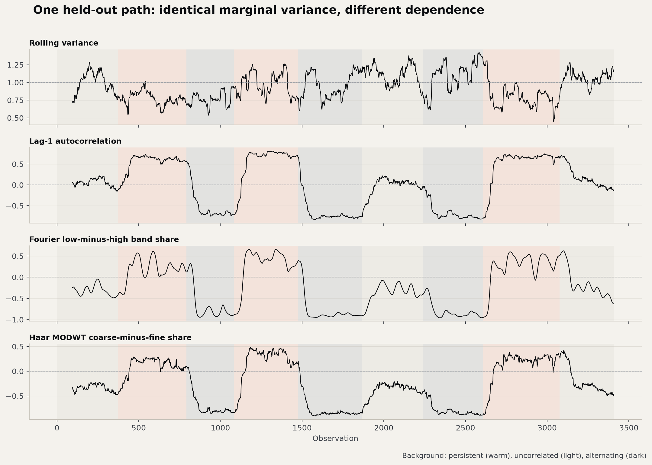
For this experiment, regime means dependence structure. The process moves between persistent, uncorrelated, and alternating states while preserving the same unconditional variance in every state. That separates the texture of the series from its overall amplitude.
The construction is a piecewise AR(1) process:
where is the known state and
| State | Interpretation | |
|---|---|---|
| Persistent | Successive observations tend to retain their sign and direction. | |
| Uncorrelated | No lag-one dependence. | |
| Alternating | Successive observations tend to reverse sign. |
Because the innovation standard deviation is , every segment has stationary variance one:
The state therefore changes without a designed change in marginal variance. A variance-only detector is being asked a precise question it should not be able to answer reliably.
Experimental design
The benchmark uses 30 generated paths for calibration and 120 independently seeded paths for testing. Every path contains nine segments, balanced across the three states. Segment lengths are drawn uniformly from 288 through 480 observations. Features are calculated from a trailing 96-observation window, so every value available to the classifier at time comes from time or earlier.
The calibration and test random seeds are fixed and different. No test path is used to choose a feature, band, classifier, or threshold.
Four feature families are compared:
- Rolling variance. The logarithm of the variance inside the trailing window.
- Lag-one autocorrelation. The sample correlation between adjacent values inside the trailing window.
- Fourier band shares. A Hann-tapered periodogram divided into four fixed bands with edges at , , , , and cycles per observation. Band powers are normalized to sum to one.
- Haar MODWT shares. Four maximal-overlap Haar detail levels plus the remaining scaling energy, normalized to sum to one. Periodic extension is confined to the already-observed trailing window.
The Fourier and MODWT features are both scale distributions. For either one, the normalized energy at band or level has the form
That normalization removes total amplitude from the feature and preserves how energy is distributed across scales.
Each feature vector is standardized using calibration-set means and standard deviations. A nearest-centroid classifier is then fitted to stable calibration observations. There is no model-specific tuning: the classifier assigns a test feature to the closest calibration centroid,
The classifier is intentionally plain. The experiment is testing whether a feature exposes the known state, not whether a flexible learner can recover it after enough fitting.
The scorecard
No single metric answers whether a regime detector is useful. This benchmark reports four:
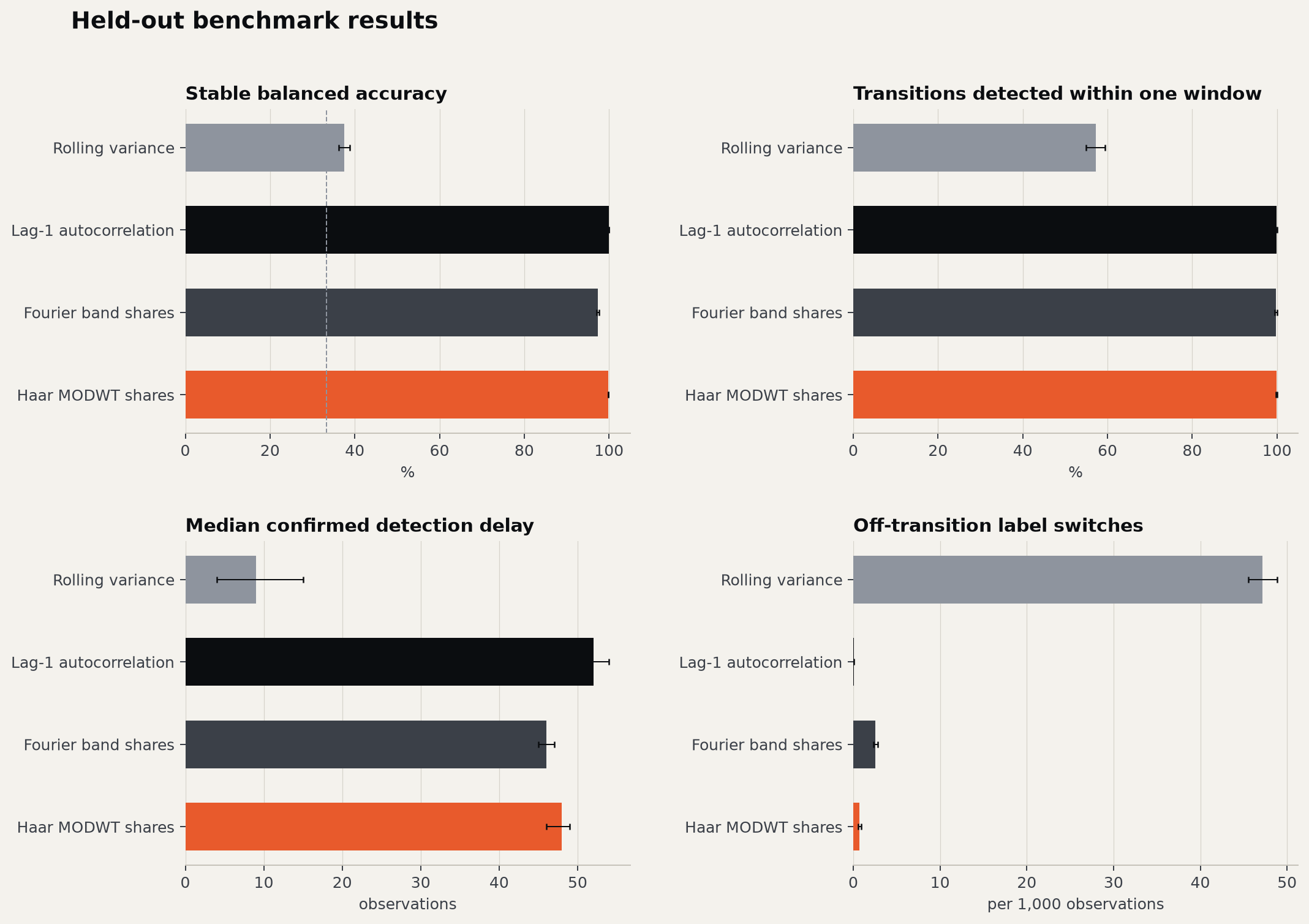
- Stable balanced accuracy. Mean recall across the three states, measured only after one full 96-observation window has elapsed since the latest true transition. Chance performance is .
- Transition hit rate. The fraction of true transitions for which the new state appears within one trailing window. Confirmation requires the target state on at least eight of ten consecutive outputs.
- Confirmed detection delay. Observations from the true transition to the first confirmed output. This is reported only for transitions that were detected.
- Off-transition switches. Raw label changes per 1,000 stable test observations. This exposes detectors that manufacture low latency by changing their answer repeatedly.
Intervals are nonparametric 95% bootstrap intervals from 4,000 resamples. Path-level metrics are resampled across the 120 held-out paths; detection delay is resampled across detected transition events.
Results
State recognition
| Feature | Stable balanced accuracy | Hit within 96 |
|---|---|---|
| Rolling variance | 37.55% [36.23, 38.81] | 57.19% [54.90, 59.38] |
| Lag-1 autocorrelation | 99.99% [99.98, 100.00] | 99.90% [99.69, 100.00] |
| Fourier band shares | 97.37% [97.07, 97.68] | 99.79% [99.48, 100.00] |
| Haar MODWT shares | 99.83% [99.76, 99.89] | 99.90% [99.69, 100.00] |
Transition behavior
| Feature | Median confirmed delay | Off-transition switches / 1,000 |
|---|---|---|
| Rolling variance | 9 [4, 15] | 47.17 [45.51, 48.84] |
| Lag-1 autocorrelation | 52 [51, 54] | 0.05 [0.02, 0.10] |
| Fourier band shares | 46 [45, 47] | 2.55 [2.30, 2.79] |
| Haar MODWT shares | 48 [46, 49] | 0.71 [0.54, 0.91] |
The simple baseline wins
Lag-one autocorrelation is effectively perfect in the stable portions of this test. That is the expected result, not an embarrassment for the other methods. The hidden state is defined by the lag-one AR coefficient. If sample autocorrelation did not recover it, either the experiment or the implementation would need investigation.
This is why a benchmark must include a canonical method matched to the claimed signal. A more elaborate detector does not earn credit for rediscovering a quantity that a direct estimator already measures.
Fourier and wavelet energy see the same structure
Fourier band shares and Haar MODWT shares both recover the state with high held-out accuracy. That is also expected. Positive serial dependence moves spectral mass toward lower frequencies; negative dependence moves it toward higher frequencies. Fourier bands and wavelet levels organize that second-order structure differently, but they are not competing theories of the data.
In this setup, Haar MODWT is more stable away from transitions, while the Fourier feature confirms transitions two observations earlier at the median. Those differences belong to this generator, window, and feature definition. They are not evidence that either representation is universally better.
Fast can mean unstable
Rolling variance reports a nine-observation median delay among the transitions it detects. Read alone, that number makes it look like the fastest method in the table. The rest of the scorecard changes the interpretation:
- It detects only 57% of transitions within the allowed window.
- Stable balanced accuracy is only modestly above chance.
- It changes labels about 47 times per 1,000 stable observations.
Its short conditional delay is largely an artifact of frequent switching. A detector that guesses constantly will sometimes guess the new state quickly. Latency without hit rate and false-alarm behavior is not a performance claim.
What carries over to market research
The numerical values do not carry over to markets. The research discipline does.
Define the state before selecting the transform. A volatility-level regime and a dependence regime are not interchangeable. Neither is a proxy for trend, liquidity, or tail risk unless that relationship is separately demonstrated.
Use a baseline that can falsify the complicated method. Here, autocorrelation is the direct estimator. In another experiment it might be a rolling realized-volatility estimator, an ADX-style trend statistic, or a parametric state-space model. The baseline should be strong enough to win.
Keep the feature causal. Centered filters, symmetric smoothing, revised historical labels, and boundary coefficients can quietly introduce future information. Every feature in this benchmark uses a trailing window only.
Separate state recognition from transition prediction. This experiment tests whether a method recognizes a change after it begins. It does not test whether the method forecasts the transition. Detection and prediction require different targets and different evidence.
Fit on one set of paths and report another. Thresholds or centroids chosen on the same history used for scoring produce an optimistic estimate even when the feature itself is causal. Walk-forward market evaluation is harder than the held-out synthetic split used here, but the principle is the same.
Report the failures. Rolling variance is included because its failure is informative. A research report that contains only the winning chart does not show whether alternatives were tested seriously.
What this experiment does not establish
This benchmark does not show that:
- any feature predicts market returns or regime transitions;
- wavelet features produce trading alpha;
- AR(1) states are an adequate model of financial markets;
- Haar is an optimal wavelet for market data;
- a 96-observation window is a production default;
- the results survive stochastic volatility, jumps, heavy tails, changing correlations, microstructure noise, or transaction costs.
The synthetic process is intentionally easy. That makes it a unit test for the measurement layer. Passing it is evidence that the feature responds to the kind of scale structure it claims to represent. It is not evidence that the same feature solves the market problem.
Reproduction
The complete generator, feature extraction, classifier, metric definitions, fixed seeds, and plotting code are available in the benchmark script. The unrounded aggregate output is available as CSV and JSON.
The implementation requires Python 3.11 or newer, NumPy, and Matplotlib:
python benchmark.py
This public benchmark is separate from MorphIQ Labs' proprietary comparative market-regime research. It contains no market dataset, private transform ranking, production threshold, or product configuration.
References
- James D. Hamilton, "A New Approach to the Economic Analysis of Nonstationary Time Series and the Business Cycle", Econometrica 57(2), 1989.
- Donald B. Percival and Andrew T. Walden, Wavelet Methods for Time Series Analysis, Cambridge University Press, 2000.
- Peter D. Welch, "The Use of Fast Fourier Transform for the Estimation of Power Spectra", IEEE Transactions on Audio and Electroacoustics 15(2), 1967.
- Kay H. Brodersen et al., "The Balanced Accuracy and Its Posterior Distribution", 20th International Conference on Pattern Recognition, 2010.
- Charles Truong, Laurent Oudre, and Nicolas Vayatis, "Selective Review of Offline Change Point Detection Methods", Signal Processing 167, 2020.
For the scale-energy construction that motivated this benchmark, see Wavelet-Domain Regime Detection with the MODWT. For property-specific tests of SWT, SSWT, the EMD family, VMD, and EWT, see Advanced Signal Decompositions Need the Right Test.
More from Quant Research
August 6, 2026 · 11 min
Advanced Signal Decompositions Need the Right Test
SWT, synchrosqueezing, EMD, VMD, and EWT are often placed in the same comparison table because they all decompose a signal. That makes them look like interchangeable candidates for one job. They are not.
August 6, 2026 · 4 min
How Spread Foundry Uses Regime Context
A regime label is a compressed description of recent market behavior. It is not a forecast, and it is not a trade.
July 6, 2026 · 2 min
Options Spread Analytics Should Be a Workflow, Not a Table
Most options tools start with a table. Rows of contracts, columns of Greeks, filters, probabilities, and implied volatility fields. The table is useful, but it is not a decision process. A trader still has to assemble…